How to work with formulas in Excel

Originally the objectives that had been pursued at creating spreadsheets were basically aimed at using formulae. Let's regard this mechanism in detail.

What to do to make the program distinguish that there is not just a common value in a cell, but there is a formula? In order to do this one must enter it from the sign of equality (=).

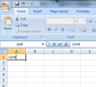
Let's try to consider the following example. Let's make the cell A1 active and enter =2+6. Input of this information is displayed in parallel in the formula bar.

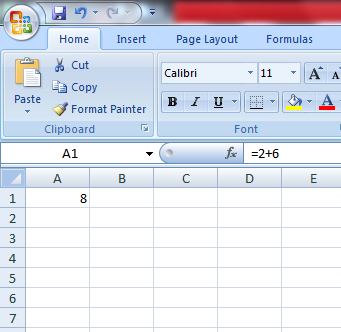
Now press the Enter key. In the cell A1 the result will be displayed (8), and in the formula bar a formula will be displayed.

Let's try to input different arithmetical operators: (+) addition, (-)subtraction, (*)multiplication, (/)division. In order to use them correctly, one have call to mind school mathematics. First one must work out the parentheses. Multiplication and division are calculated before making addition and subtraction. If the operators have the same priority, then the calculations are carried out alternatively, from left to right.

We advise you to use parentheses, as you will be protected from a mistake, besides, it will make the process of reading and analyzing formulae easier. You can use any number of parentheses, though, if there is a discrepancy in the number of opening and closed parentheses, so the program will report an error, and will give the variant for correction. When you input the closing parenthesis, the last couple of parentheses are displayed visually. It makes the use of significant number of parentheses convenient.

Formula let make cell references. Let's consider an example.

Fill the cells with data: А1 - 5, А2 - 10, and fill the cell А3 with the formula =А1*А2. Press Enter. In the cell A3 there will be product of the cells A1 and A2. Let's change the value of the cells A1 and A2. Let's take notice of that, so you see that the value of the cell A3 will be changed automatically

It's complicated enough to input addresses of cells (C4, D3, etc.), that's why it's often more convenient to use a mouse for input of references. If we want to use a mouse, then we make the following steps. We make the cell A3 active, then input the sign of equality (=). Click on the cell A1, input the sign of multiplication (*), click on the cell A2 and press Enter.

As you see, the result is the same.

There are relative, absolute and mixed references:

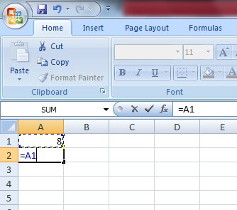
• Relative reference - this is indication at the cell, relative to its location to the cell with a formula. It's designated - A1.
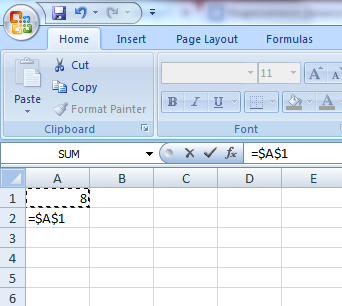
• Absolute reference - this is indication at the cell with unaltered location. It's designated - $A$1
• Mixed reference - this is variation of relative and absolute references - $A1, A$1.

In order to change the type of reference, one should use the key F4. Let's consider an example. Fill the cells: A1-20, A2 - formula=A1. Now press the key F4. The type of reference is changed each time you press the key F4.

 

Now let's see how all these references differ.

To see this, first fill the cells in the following way: – 10, А2 – 20, В1 – 100, В2 – 200. And input the formula =А1+А2 in the cell A3. Now press Enter.

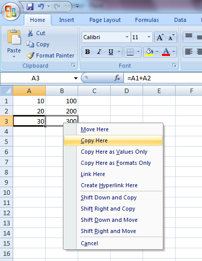
Place the cursor in the lower right corner of the cell A3, on a small black square. Click the right mouse key and drag on the cell B3. Release the mouse key. The context menu appears. Choose from this menu "Copy cells"

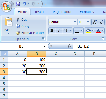
Value of the formula from the cell A3 has been copied to the cell B3. Make the cell B3 active. In the formula bar there is a formula: =А1+А2. Our formula in the cell A3 has been recorded =А1+А2, Excel gets it like this: "It's necessary to take the value from the cell, located two rows above in the same column, and add to it the value of the cell, located one row above, also in the same column." These are relative references. If we copy the value of the formula from the cell A3 to C3, then we would get =С1+С2.

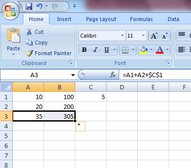
Let's regard absolute references. Leave the data of the cells А1, А2, В1, В2 the same. Delete the value of А3 and В3. And input number 5 in C1.

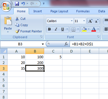
In the cell A3 input the formula =А1+А2+$C$1. And now copy this formula to the cell B3, as we made it just now. Make the cell B3 active. Relative references have been changed to new values, and absolute reference has stayed the same.

Let's regard mixed references. Fill the cell A3 with the formula =А1+А2+C$1, copy it to B3. In B3 the formula =А1+А2+D$1 has appeared. i.e. the number of the row is unchanged, but the letter of the column is relative, that's why it's adjusted to our operations.

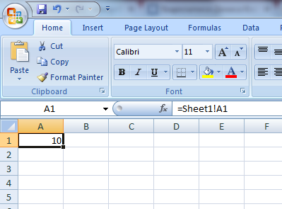
It's also possible to refer to other sheets of the book (we are talking about the external reference). Let's consider an example.

For example, we want to write in the cell A1 (Sheet 1) the referenced cell A4 (Sheet 2). Select the cell A1, input the sign of equality. Now click on the tag "Sheet 2" and on the cell A4. Press Enter. Look what we have got. In the formula bar of the cell A1 on Sheet 1 has appeared the formula =Sheet1!А1

If we input the reference from another book, then it will look like this: =[Book2]Sheet1!А1

In order to edit the formula, activate the cell which keeps this formula, so make double click on it. Now it's possible to edit it. In order to fix the changes, press Enter.

A text should be placed in double quotes. For example, ="$55"+$"33". The formula like =$55+$33 will be not correct.

The program changes a text into a numeric value. That's why the sum of the specified formula will be a result 88.

In order to combine text values, an operator " (ampersand) is used. For example, if the cell A1 has the value "Arun", and the cell A2 has the value "Kumar". If we input the formula =А1&А2 in the cell A3, then we will get the value "ArunKumar". If you need a space between the name and the family name, then you should write in the following way: =А1&" "&А2.

Ampersand is also used for combining the cells with different types of data. For example, combining the cells with the values 10 and apples, the result of the formula will be text value "10apples"